(click here to enlarge)
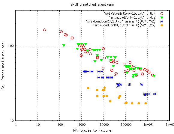
Fig. 1: Stress amplitude vs. Cycles to failure
The present study outlines a fitting process applied to SRIM composite data[2], that has proved reasonably successful for another reinforced plastic [3]. Load control and strain control test results for different R= (Smin/Smax) loading are displayed in a Neuber Stress[4] plot and sets of Stress-Strain-Life points are used to characterize the cyclic stress-strain and fatigue behavior.

(click here to enlarge)
Fig. 1: Stress amplitude vs. Cycles to failure
As one would expect with the variation of R ratio of the data sets, the combined plot shows a great deal of scatter and suggests that stress amplitude alone is not a good overall indicator of fatigue life.
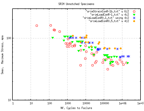
The plot of maximum stress versus cycles to failure is a substantial improvement in collecting the data points into a single, predictable band, but there is still substantial scatter:
(click here to enlarge)
Fig. 2: Maximum Stress vs. Cycles to failure
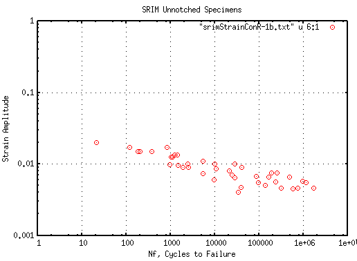
Three of the data sets were results of load control tests. If one plots only the strain controlled tests results the scatter band is substantially narrower, although there is obviously also a Y-axis scale change effect. No measurements of strain amplitudes were reported in the results however for the load control test sets, so it is not possible to plot both strain control and load control results in a strain amplitude plot.
(click here to enlarge)
Fig. 3: Strain vs Cycles to failure for strain controlled tests
The strain life data in standard SAE format is available here:
      SRIM standard(SAE) strain-life data file
      (Some extra columns of calculations have been added in each row.)
Plastic strain values have been computed by the equation
Plastic_Strain = Total_Strain - ( Stress / E )
As one can see in the file the calculation yields negative numbers.
This discrepancy is due to the scatter in the "elastic modulus" of
the individual tests. The effects is documented in ref.[5] for
another material, but in brief, one can attribute this scatter in
modulus to non-fully random patterns of fiber placement in each
specimen, and to change in "elastic" modulus of the plastic
matrix as each fatigue test progresses. One could measure each
test's cyclic modulus to assist in the computation of plastic
strain, but often such initial and cyclic modulus measurements are
not made or reported in tests, and it is easier to adopt alternate,
simpler, methods of fatigue curve fitting analysis.
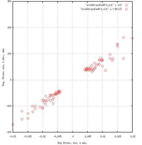
In the plot of the cyclic stress-strain curve both the tensile tip and the compressive tip of the stabilized stress-strain hysteresis loop is shown:
(click here to enlarge)
Fig. 4: SRIM Cyclic Stress-Strain results for strain
controlled tests.
Composite materials are not necessarily as symmetric (tensile shape versus compression shape) as metallic materials, hence the separate plot to check if this difference is the case in the present data. The plot also indicates the degree of scatter and also the overall lack of apparent plasticity. It is possible that on a local scale of fibers and surrounding matrix, that there is much greater plastic behavior in at least the matrix, but there presently is no reasonable way of measuring such a deformation. For the curve fitting purposes of this study boundary lines were drawn around the cyclic stress-strain data. A median line was then drawn between the boundary lines. Two of the data points that fall outside of the boundaries on the tensile side had large mean stresses and have been excluded from this fit.
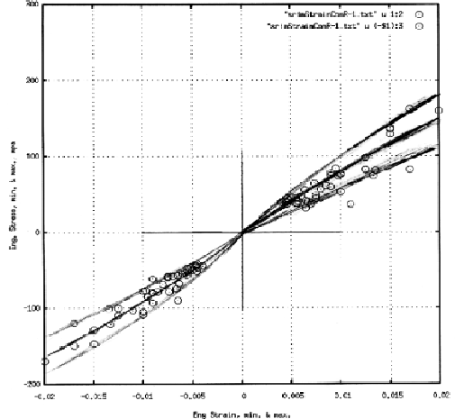
(click here to enlarge)
Fig. 5: Tensile and compressive cyclic stress-strain
data and boundary curves.
A median curve was then drawn between the boundary lines and digitized with several stress-strain values.
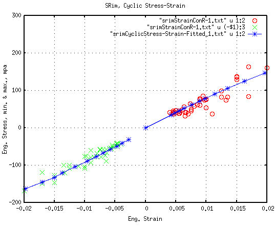
(click here to enlarge)
Fig. 6: SRIM Cyclic Stress-Strain data and digitized fitted
curve (blue).
At this point in the fitting method we have set or defined the relationship between cyclic stress and cyclic strain. We still need the life term to define the complete triplet. In a past study
Reinf. Polypro.
the strain life curve was used to determine the missing life term. This
option is also usable here, but it would be an advantage to also incorporate
the load control test results. This can be achieved by plotting
the strain control tests and the load control tests in a Neuber plot.
Strain control test results are plotted versus fatigue life, using the
energy parameter:
      Sneuber_Ampl. = SQRT ( Sa * Strain_Ampl. * E )

where
      Sa is the stress amplitude of the stress-strain hysteresis loop

      Strain_Ampl.  is the strain amplitude of the loop

      E   is the elastic modulus
In the present study the elastic modulus is measured from the fitted
cyclic stress-strain curve shown in figure_6, and has a value of E=8600_mpa.
The result for the SRIM strain controlled tests is depicted as the open red circles in figure_7. The constant amplitude load control tests are also plotted in the same graph with an equivalent stress amplitude versus life. For the load control tests the equivalent stress amplitude was calculated using the equation:
      Sequiv_Ampl  =   SQRT ( Smax  * Sa )

where
      Smax is the maximum stress of the load control test

      Assumption:  tests are predominently elastic
The formula is basically the same as the one for Sneuber_Ampl above,
and under fully reversed loading reduces to the same equation.
By using "Smax" one introduces a form of mean stress correction
similar to the one commonly used in past[6].
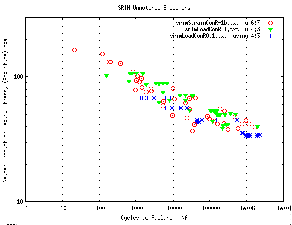
(click here to enlarge)
Fig. 7:Plot of Neuber stress for strain life results and
an equivalent stress for load control tests versus life.
Figure 7 gives a good combined plot of the results, although there is still the usual large amount of scatter typical of composite material fatigue results.
When the data for load control tests with stress ratio of R = 0.5 is added to fig. 7 the result, as shown in figure 8 are not as satisfying, though probably still better than the plots of figures 1 and 2.
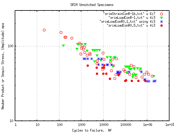
(click here to enlarge)
Fig. 8:Neuber plot for strain control and load control
R=-1, R=0.1, and R=0.5
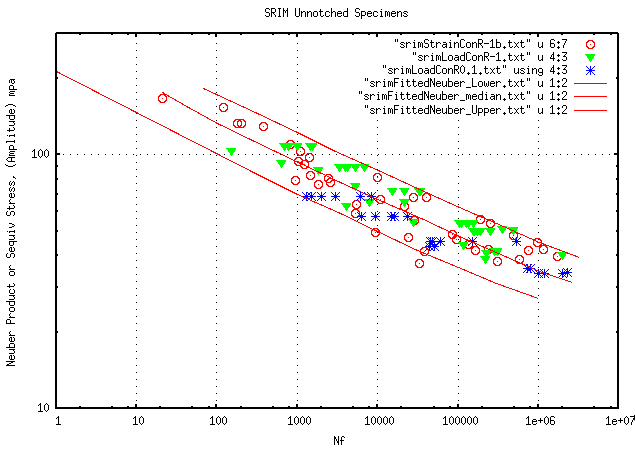
One could speculate that the considerably higher mean stresses of R=0.5 stress control tests, and the lack of strain control, would cause substantial cyclic creep to occur during the fatigue tests; thereby introducing a different failure mechanism. It was decided to leave the R=0.5 tests out of the fitting process. Using Fig.7 above, a lower and upper boundary line was drawn (sketch available here) and followed by a median curve between the two boundaries. The sketched lines were then digitized and are shown in Fig.9.
(
click here to enlarge)
Fig. 9:Neuber plot with fitted boundary and median lines.
For comparison purposes the load control R=0.5 data was superimposed on the fitted plot above and is available here: Addition of R=0,5 data to Fig.8
A summary page of the results for SRIM is available:
SRIM Fatigue Data Web Page
The page also includes three fatigue life calculators that use
the three fitted curves above. One can use them to estimate fatigue
life given inputs of calculated Finite Element elastic stress.
The calculator program, implements the Neuber plasticity correction to
obtain local stresses and strains prior to computing fatigue damage,
and is the same as used for all the metals in
the
FDE_fatigue_data.
The validity of using a Neuber type plasticity correction for composite
material life prediction is not yet clear, however.
In this study it was also found that, when the apparent stress-strain behavior is predominantly elastic, one can use a variation of the Smith-Watson-Topper mean stress parameter to enable a unification of specimens results tested under different cyclic R ratios into a Neuber parameter plot.
One can conclude from the study that it is possible to fit calculation curves to the three fatigue variables Stress, Strain and Life, without the necessity of dividing total strain into plastic and elastic components. A cyclic stress-strain curve and relationship to fatigue life based on either energy or strain appears to provide sufficient information for an adequate fit in materials that are difficult to process with traditional fitting methods.