Using a Material Deformation Model to Predict Bending and
Axial Straining Effects in Coiled Tubing
A.Conle Univ. of Windsor
Apr. 14 2015, Updates: May 5-10
Copyright (C) 2015 A.Conle
Permission is granted to copy, distribute and/or modify
this document under the terms of the GNU Free Documentation
License, Version 1.3 or any later version published by the
Free Software Foundation; with no Invariant Sections, no
Front-Cover Texts, and no Back-Cover Texts.
A copy of the license is available here:
"GNU Free Documentation License".
( "http://www.gnu.org/licenses/fdl.html" )
Introduction:
Coiled tubing is extensively used in oil and gas well
applications to perform tasks such as well logging,
machining at depth, etc. Examples of operations are
described in Refs.[1,2]. Generally a long steel tube of
1 to 4in. (25 to 100mm) diameter is wound onto a spool and
transported to the well site. At the well site the tube is
straightened/bent several times as it is inserted into the
well or water (offshore well service) and then re-spooled.
Due to the large strains imposed on the tubing considerable
fatigue damage is imposed on certain sections of the tube
during each operation and consequently the tube is designed
for a finite life of a few hundred operations.
The present work describes the application of a
cycle-by-cycle material deformation model[5] to a set of
similar sequences as encountered in a reel/unreel/re-reel
event of a coiled tube. The model does not account for
internal pressurization events nor for torque events on
the tube while in the simulated service, but is only
used here to follow the distribution of stresses and
strains of a single tube section. It is hoped that the
simulation will enable students to better understand the
plastic deformation, residual stresses, and fatigue of
tubes subjected to combined bending and axial strains,
and to help design engineers to envision the tube behavior
during well intervention operations.
The simulation program, available to anyone interested,
is written in Fortran under an "OpenSource" distribution
license. The author hopes that the program structure
will encourage other researchers to add code for tube
pressurizations, torque rotations, and contact stresses
which require cognizance of Multiaxial deformation and
fatigue that are beyond the scope of this presentation.
 (Click figure to enlarge)
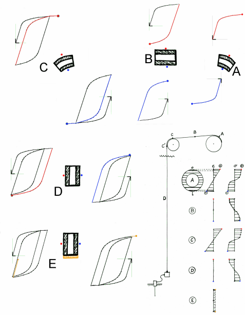
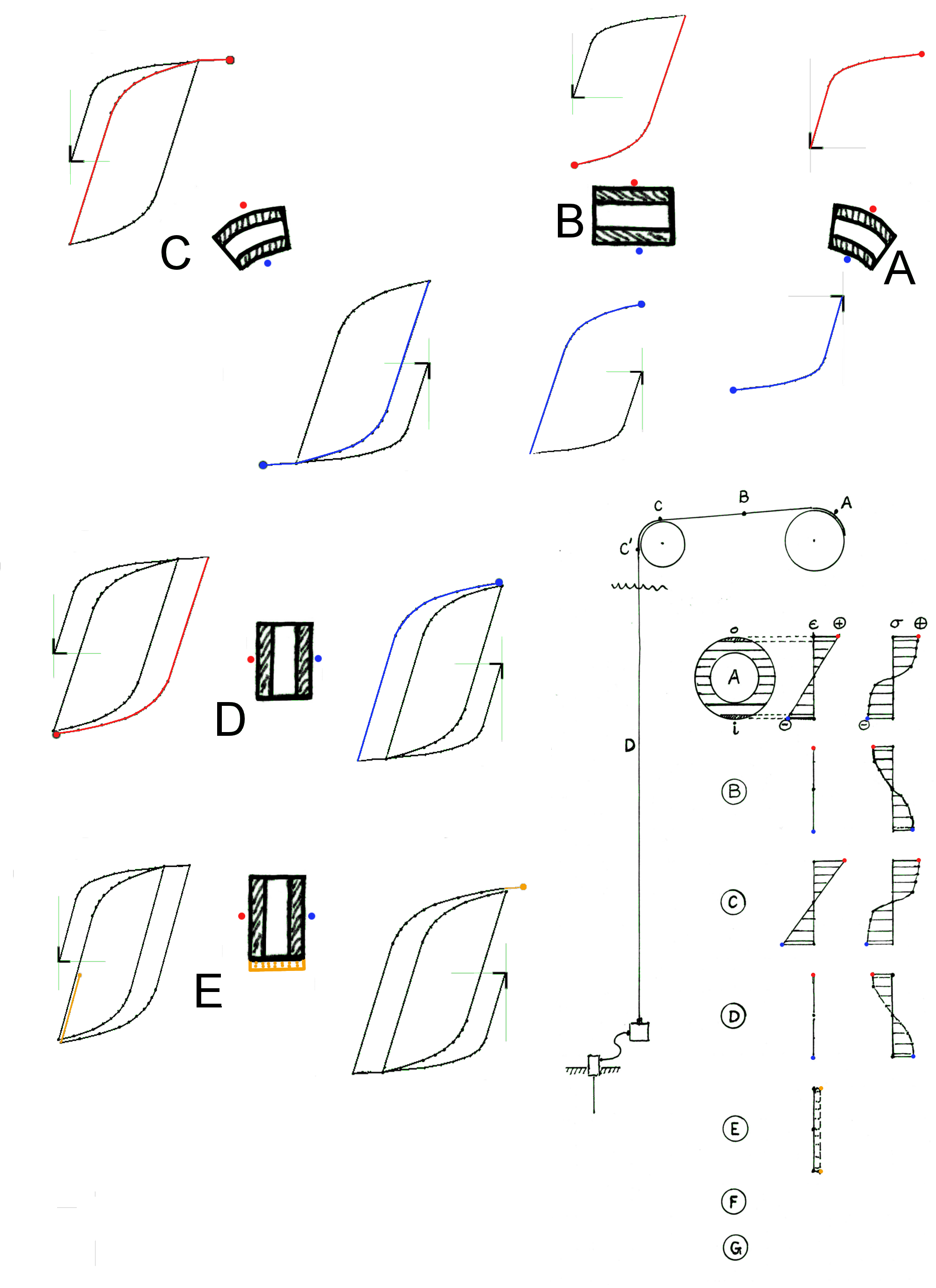
Fig. 1: Schematic of extreme fiber stress-strain response
during an off-shore coiled tubing operation
Assumptions and Starting Points:
- The stress-strain model uses a push-down list or
"last in - first out (LIFO)" system to account for
material memory events [5].
- Masing's [4] hypothesis regarding the shape of
the stress-strain hysteresis loops is adopted. It
presumes that the shape of stress-strain hysteresis
loops is similar to the cyclic stress-strain curve
shape, but both stress and strain values multiplied
by a factor of two.
- Cyclic hardening and/softening are not modelled.
- Cyclic stress relaxation and cyclic creep are not modelled.
- Tube cross-sections remain plane during bending and
axial straining events.
- Multiaxial loading is not modelled; only bending and
axial tube straining effects are simulated.
- The simulation assumes that the tube is discretized into
a series of elements or layers with enforced compatability
at each layer edge (plane sections remain plane in bending).
A separate uniaxial stress-strain model is used
to simulate each layer's cyclic stress-strain behaviour, with
the point of modelling at the top and bottom of each layer.
Material:
Due to a lack of published tube steel fatigue information
in the literature the present study used the cyclic deformation
and fatigue properties of HSLA-350 (or SAE950X) published from
research on ground vehicle steel.
 (Click figure to enlarge)
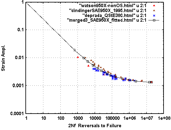
Fig. 2 : Strain-life fatigue data and fitted curve
for merged files of HSLA-350X (SAE950X) steel)
Data file is available
here.
In the following analysis sections the local stress-strain
and fatigue life estimations utilize the "Fitted" curve (black lines)
shown in Fig. 2 above. These fitted data points are available in the file:
Bending and Axial Stress-Strain During a Coiled
Tubing Operation
In an off-shore coiled tubing operation the tube is
initially spooled onto a large reel on the ship. For a
given point along the tube the strains are primarily in
bending as shown in Fig._1 at point "A". There are also
stresses imposed as the tube sits on the reel, but these
are not considered here.
The stress-strain patterns shown at "A" are for the maximum
and minimum strain points at the tube section. In the
"layered" section approximation, shown in the lower right
of the figure, the maximum strain point would be at the
top of the section which corresponds to the tube section
point the furthest away from the reel. Similarly the
most negative compressive stress-strain would occur at the
bottom of the section shown (closest to reel). Given that
cross-sections will remain planar during bending, the
approximate stress and strain distributions across the
section are also depicted at point "A" in the lower right
portion of the figure.
During an operation the tube is uncoiled from the reel
"B" (and straightened), then bent over a sheave ( "C"),
then straightened("D") as it enters the well or water.
In on-shore applications the tube is straightened,
as it comes off the sheave, by overstraining in the
outward (of sheave) direction to allow for spring-back.
Off-shore applications may not add this step and instead
use an end-weight to keep the tube straight in the water.
The over-bending to avoid spring-back step has not been
added to the strain history in this study for simplicity
reasons.
Fig. 1, in the lower right section, depicts in schematic
form the stress-strain behavior at the maximum and
minimum bending strain points and the corresponding
cross-section stress and strain distributions. Due to
self-weight additional axial strains may be imposed on
top of the bending history. Wave action too will add
smaller bending and axial strain cycles near the sheave.
In addition to the axial and bending strains, operations
will also impose pressure and possibly torsional stresses
and strains on the tube which will lead to multiaxial
states of straining in parts of the tube. Multiaxial
stress and strain effects will not be covered in this
study. Ovalization, wall thinning and tube lengthening
due to cyclic ratcheting are also not discussed here.
Defining a Strain History Table:
In coiled tubing applications the bending strains
are quite large and are well into the plastic zone
of material deformation. Large strains of this size
when imposed on axial samples cause very short fatigue
lives and the service life of a coiled tube is similarly
short; of the order of a few hundred operational cycles.
For fatigue life prediction it becomes necessary to
track the stress-strain history of each tube segment,
as each service operation may require a different tube
length to be uncoiled/coiled, and the critical fatigue
"hot spot" location on the tube varies from job to job.
Tracking the strain history of each segment can be done
in tabular form and the format used to feed the strains
into the stress-strain simulator in this study is shown
in example file:
strains1.txt
The features of the table used in the simulations are
- Material file name: relates the fitted variables
strain, stress, and fatigue life and data lines,
- Comment lines starting with a "#" character
- Data lines: in this case case 9 columns, that
include a time stamp, the membrane strain
(uniform section strain), the bending strain,
tube pressure, position, and 4 tube diameter
dimensions.
In the simulation only the time stamp and membrane (em)
strain and bending strains (eb) are used. A simple on-line
"demo" version of the model is available here:
https://fde.uwaterloo.ca/Fde/Notches.new/memoryExample.html
It shows a simple sequence of strain for an HSLA 50ksi
material, and a version that allows user input is
available here:
https://fde.uwaterloo.ca/Fde/Materials/Steel/Hsla/Merged950X/merged3_SAE950X_sim.html
Simulation Software
The main stress-strain and fatigue simulation routine used
for each layer interface is the program "pdStressStrain.f".
It reads an input file like the one detailed above, and
computes the stress-stain and fatigue damage response.
Several other routines then take its output file and
create plots of stress and strain distributions, stress-strain
hysteresis loops, and stress-strain energy per layer.
- pdStressStrain.f
Stress-Strain Simulator. Given a strain history (em + eb)
and a fitted strain-stress-life file, computes the
stress-strain response and the fatigue damage on a
half-cycle by half-cycle basis.
- runLayers
bash script(Linux) which scales the input bending
strain according to each layer edge of the tube
cross-section and then run pdStressStrain for that
edge. Produces the stress-strain histories of each
layer edge.
- plotLoops
bash script to plot data from two runs of pdStressStrain.f
e.g. the stress-strain histories for both points
at max and min points of the tube cross-section.
- computeAreas.f
Used to compute the cross-sectional areas of each
of the "n" layers of tube cross-section.
- deltaEvents.f
Given the (strain stress time) input from pdStressStrain.f
output file, program extracts the items between event1
and event2. Also puts out energy computed from the
stress-strain sequences.
- delete1arg.f
Used to delete 1st string (in this case ID tag) from line(s).
- reportEvent
Script to plot the stress and strain distributions at
end of a event.
- report2events
Script plots stress and strain distributions at
event_1 and event_2 and the stress strain paths
of max min layer edges between the events.
-Also makes delta energy plot: energy imparted by
cyclic deformation.
- The above computer routines can be found here:
https://github.com/pdprop/pdStressStrain/tree/master/CleanPDSS
(Note: Click on the program name, then
Click the "Raw" button to download individual files)
or
To download a tar file of all the above files go to:
https://github.com/pdprop/pdStressStrain
and Click on the file "allfiles.tar" then
Click on the "Raw" or "View Raw" links to download.
- Other software needed for Linux: gnuplot, htmldoc
and xv which are used to automate the reporting process.
A Fortran compiler like "gfortran" is needed to compile
the *.f programs.
In the following sections of this web page some of the
typical states of stress-strain sequences and the resulting
stress and strain distributions for events at "A", "C" and
"D" (as per Fig.1) are displayed. The strains imposed
are only rough estimates of what one may expect and have
not been measured from actual service.
Stress-Strain at "A"
After production a length of coiled tube is wound onto the reel
for transport to various job sites. The reel is often larger
in diameter than the sheave and thus it has been assumed for
this demonstration tube section, that the reel bending strain
has a value of 0.008 at the outer tensile surface of the tube.
For an HSLA 50ksi material this strain is well beyond yield.
In this case the initial "monotonic" or tensile/compression
curve of the virgin material has not been modelled. For initial
loading the cyclic stress-strain curve has been applied. Most
HSLA materials do not have significant cyclic hardening or
softening, and consequently the cyclic curve should be reasonably
close to the monotonic stress-strain behavior. In the strains1.txt
file the state of "A" (Fig.1) is denoted by first column
time stamp "601." %nbsp Figure 3 shows stress-strain sequence
plots of the two extreme fiber locations.
The blue line/points simulates the stress-strain path of the
compression side of the tube as the pipe is wound onto the reel
and the red simulates the extreme fiber of the tensile side of
the bent tube.
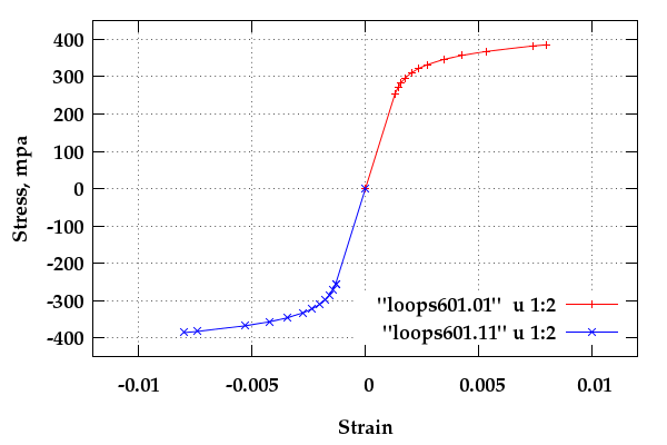
Fig. 3: Stress-strain path of two extreme fibers on
surface of tube as section is wound onto reel.
In a typical service operation the tube will be unwound from
the reel (straightened somewhat) and passed over the sheave
into the water (bend to sheave radius, then straightened again).
A typical simulation output file (text) for LayerEdge 1 can
be viewed here:
The fatigue damage up to timestamp 2062.19 can be extracted
using the command:
     grep TOTDAM  layerEdge.01.2062.19.out.txt

with result:
     #TOTDAM90=  0.5774353E-03 allowed Repeats= 1731.8   nrev= 6

and similarly the stress-strain history leading up to that time
can be extracted for plotting with the command:

     grep \#plotloops layerEdge.01.2062.19.out.txt | delete1arg > loops.01
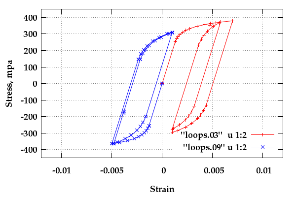
Figure 4 plots the history of the stress-strain path of
the two extreme fibers as the segment of interest comes off
the sheave (point C', or timestamp 2062.19 ).
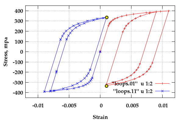
Fig. 4: Stress-strain path of two extreme fibers on
surface of tube as the section exits sheave.
The script "runLayers" above is used to automate the
simulation for all LayerEdges and produce a set of stress-strain
plots:
When all the stress-strain loop files for a given timestamp
exist, their last(in file) stress-strain points can be plotted
to show a stress distribution and a strain distribution at each
LayerEdge across the section:
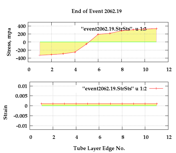
Fig. 6: Cross-section stress and strain distributions
at layer edges after timestamp 2062.19
The linux bash code to perform this latter function is
described in script "reportEvent". Note that the bending
strain is zero at this point, but there is a slight axial or
membrane strain due to tube loads. Similar states of stress
and strain would be maintained as the tube is lowered to the
service level. In consequence significant residual stresses
remain in the tube even-though it has been straightened.
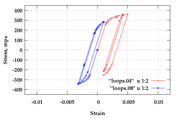
Adding Wave Action:
If the service application being performed from a ship there
will be a relatively smaller(hopefully) strain history
imposed as the surface platform moves up and down due to
waves. There will also be stresses and strains imposed due
pressurization, but pressure effects are not covered in
this study. At point " C' " both axial and bending
strains will change due to wave action. At point " D "
the majority of the wave induced strains will be assumed to
be membrane strains only. Both types of strains can be
simulated by inserting the wave strain pattern into the strain
logging file strain1.txt described previously, and
then running script "report2events".
In the strain1.txt logging file two example waves have
been inserted at Timestamps 2500.01 to 2568.63.
The simulation results from running command:
./report2events 2500 2568.63
are depicted in stress-strain plots in Figure 7.
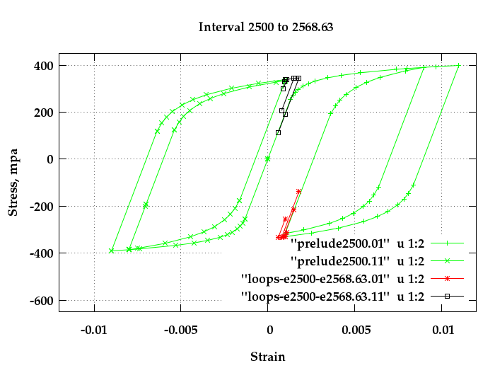
Fig. 7: Extreme fiber stresses and strains due to wave action
The stress-strain histories for these LayerEdges 01 and 11
that preceeded the waves are shown in green, and for the
waves themselves black and red lines and points are shown.
As expected the wave hysteresis loops for the example strains
are small and without plasticity. The wave effects for
LayerEdge 11 however have a very high mean stress and,
depending on their size, may cause fatigue damage.
The report2events script also produces a *.pdf format
report of the stress and strain distributions at the beginning
and end of the interval.
interval2500-2568.63.pdf
Simulating Overload Effects:
The complexity of the residual stresses and strains present
in a tube segment that arose from its past strain history
make the computation of the effects of overloads difficult.
If the residuals were not present one and normal loads were
elastic, one could just add the expected overload forces to
the present state and determine if full section yield or
other criteria had been exceeded. As shown in figure 7
most of the extended tube has approximately half its residual
stress beyond 0.2% offset yield in tension, and the other
half of the cross-section is beyond yield in compression.
One cannot simply add a force equivalent to some fraction of
yield to the existing stresses for example.
Two engineering solutions are offered to overcome this
computational problem:
    1.   Add a strain equivalent to yield strain,

         for example, to the present state of strains

         run the simulation and observe if the stresses

         for all the layers have exceeded yield stress.


    2.   Estimate how much stress-strain energy the

         overload forces would cause in a virgin tube.

         Impart a simulated strain to the present state

         of stresses and strains until the  additional

         strain energy equals that of the virgin sample

         energy.
A similar process could be used by applying a plasticity
FEA model, such as Abaqus, but it is not clear if present
plasticity models can correctly follow the complex
stress-strain histories used here accurately. One compromise
solution may be to use the present simulation to estimate
the state of stresses and strains in a section and then
apply a FEA plasticity capable model to compute the effects
of various overload conditions.
In this study the two simple methods listed above (without
FEA) have been applied.
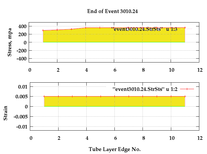
Fig. 8: Distribution of stresses and strains after
addition of an overstrain= 0.004
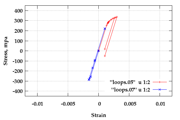
Figure 8 depicts that state of stresses and
strains after a simple overstrain of 0.004 has
been added to the stress-strain states at operation
timestamp 2568.63. The inserted overstrain is shown in log
file at timestamp 3010.24. :
strains2.txt
( The events with timestamps greater than 3010.24 have been
commented out in the file by using a "#" character at the
begining of lines.)
Figure 9 depicts the two extreme fiber (LayerEdges 01 and 11)
stress-strain changes due to the 0.004 overstrain. A strain
of 0.004 in a virgin tube would be approximately the strain
at the 0.2% offset Yield stress.
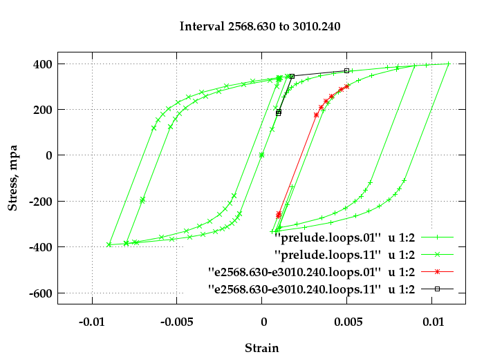
Fig. 9: Stress-strain paths before and during an
overstrain of 0.004. Timestamp 3010.240
It appears that for these assumed strains the
cross-section is at full section yield.
Application of the second method listed above requires the
computation of the stress-strain energy imparted by an
overstrain value and comparing it to some standard stress-
strain energy. The program "deltaEvents.f" performs
the energy computation function with commands such as (e.g.):
      ./deltaEvents  0   2558.630   < loops.01 > prelude.loops.01

      ./deltaEvents 2558.630 3010.240  < loops.01 > interv.loops.01
The "prelude.loops.01" file will contain the stress, strain,
and energy values leading up and including timestamp 2558.630,
while the "interv.loops.01" will contain a similar point set
for the imposed strain history from timestamp 2558.630 to 3010.240
which in the present case is the imposed membrane strain em= 0.004.
The green stress-strain lines in Figure 9 are from the "prelude"
files, and the black and red points are from the interval files.
Accumulated and delta values for stress-strain energy are
computed for each stress-strain point in these files. The
before and after energy values are subtracted and plotted
in Figure 10 for the cross-section. Values shown are
the stress-strain energy multiplied by the cross-sectional
area of each layer.
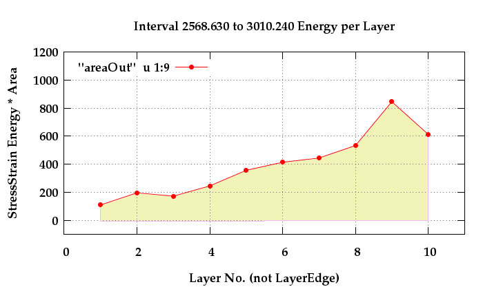
Fig. 10: Stress-Strain Energy x Area for 0.004 Overstrain Event.
The script "report2events" also produces a *.pdf summary
of the imparted energy and a detailed print of the energy per
layer:
interval2568.630-310.240.pdf
In the figure it is apparent that the side of the
tube that was in compression as it rolled over the sheave
is actually absorbing the most stress-strain energy. In this
type of energy calculation the energy is generally the area
under the stress-strain curve; as in a monotonic tension
test for example. In a cyclic loading situation the imparted
energy is the area inside a closed hysteresis loop. Thus a
virgin sample tested in tension will have net energy input
as the stress-strain rises up to some peak. Any unloading
half-cycle will actually dissipate imparted energy. This
process leads to the layer 10 imparting more energy than
layer 01 in figure 10. The overstrain event in
layer 01 is, to a large degree, an elastic unloading. Only after
its stress-strain locus crosses the zero stress axis will
the layer start to resist the external overload. Layer 10,
which is already at a high tensile stress at the start of the
overstrain, absorbs more imparted energy during the event.
Of the two above methods the simple overstrain application
and check for complete section yield is probably easier
to visualize and compute. One difficulty arises in
specifying an appropriate amount of overstrain. Perhaps
specifying an overstrain equal to some fraction of the total
strain at the 0.2% offset yield stress would suffice.
Summary and Comments:
Simulation of stress-strain behavior of coiled-tubing oil or
gas well operations for fatigue life evaluations requires
the use of a material memory model to mimic the stress-strain
paths during the complex service strain history imposed.
The present study outlines a method for simulating membrane
and bending tube deformations during an assumed operation.
Simulation results show, as expected, that large, beyond,
yield, deformations set up residual stress patterns that
must be accounted for in fatigue life calculations and for
estimating the effects of overload type events.
While working on this web page it became apparent to the
author that the low cycle fatigue information for coiled
tubing materials was very difficult to find in the literature.
Presumably the corporations that presently design coiled
tubing each have their own information. In order to obtain
an idea of the effects on fatigue of different steel heats,
material types etc. from which the industry as a whole would
draw benefit, a user and steel provider collaborative effort
to document publically their base material fatigue results
would be very useful.
Although the effects of service overload or overstrain
conditions can probably best be modelled by computing the
imparted energy and setting the allowable equal to some
standard, it is presently probably more expedient to specify
a "standard" overstrain value and then check for full
plastic yield of sections.
References:
- Wikipedia: Coiled Tubing:
http://en.wikipedia.org/wiki/Coiled_tubing
- ICoTa Publication: "An Introduction to Coiled Tubing:
History, Applications, and Benefits,"
http://www.icota.com/publications/ICoTA%20Publication%20Intro%20to%20CT.pdf
- API 17G2 Draft standard for design/use of off-shore coiled
tubing, Amer. Petrol. Industry Standards Committee, 2015
- G. Masing, "Eigenspannungen und Verfestigung beim Messing,"
in Proceedings 2nd Intern. Congress of Applied Mechanics,
Zurich, 1926.
- A. Conle, T.R.Oxland, T.H.Topper, "Computer-Based Prediction
of Cyclic Deformation and Fatigue Behavior," ASTM STP 942,
1988, pp. 1218-1236.
(An on-line presentation that outlines the memory accounting
process as applied to crack propagation is available here:
https://fde.uwaterloo.ca/Fde/Crackgrowth/fdeSpringPres2013_published.pdf )
Contact:
Author can be contacted via:
A. Conle Adjunct Prof.
c/o Prof. T.H.Topper
Dept of Civil Engr.
Univ. of Waterloo,
Waterloo, ON, Canada N2L 3G1
 (Click figure to enlarge)
 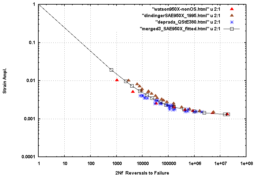 (Click figure to enlarge)
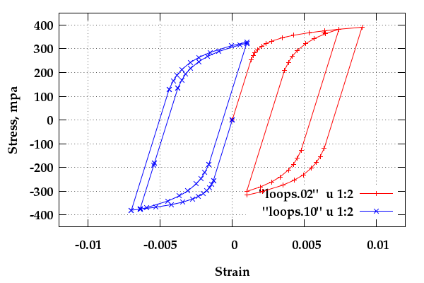