Using Finite Element Results for Fatigue Analysis: Case 2
F.A. Conle, Jan. 1 2014.
Educational Background Article
https://fde.uwaterloo.ca/Fde/Notches.new/feaFatigueCase2.html
Copyright (C) 2014 F.A.Conle and Univ. of Waterloo
Permission is granted to copy, distribute and/or modify this document
under the terms of the GNU Free Documentation License, Version 1.3
or any later version published by the Free Software Foundation;
with no Invariant Sections, no Front-Cover Texts, and no Back-Cover Texts.
A copy of the license is available here:
"GNU Free Documentation License".
( "http://www.gnu.org/licenses/fdl.html" )
Introduction:
The computation of fatigue damage in a component or larger structure where
the loading is from a variety of independent sources is more involved than the
approximations described in
Case 1.
The independence of the load histories makes it very difficult to adopt one
"worst case" load set to impose on a finite element model. A wide variety of
load sets may need to be analyzed in order to find the critical stress states
of elements. On simple components with only a few load "channels" it may be
possible to determine the significant load cases. On a structure such as an
automobile where the significant loads are buried in one or two hour recordings
from the proving grounds, and the number of independent load channels may
approach 100, the process needs to be automated (Refs.:[1,2]). The process
used is similar to that known as "Influence Factor Analysis" used for many
years in bridge construction, and the individual steps needed by the analyst
are fairly simple, but computationally intensive. An outline of the process
is given in the following sections.
Loads:
The loading on a vehicle, such as sketched in Fig.1, must generally be
determined by analysis using dynamic models such as ADAMS, from laboratory testing,
from measurements of previous prototypes, or from direct measurements from
the proving ground events. A front lower arm bushing as indicated in Fig.1
may have three forces and one or more moments as load inputs (only 3 forces are
shown).

Fig. 1:
For many vehicles similar to the one shown of a car "body in white" there are sixty
or more load or moment vectors applied to the body.
The load for each variable is calibrated to known laboratory inputs and observed using
load cells or strain gages on the body or the suspension component. With all load
channels calibrated the vehicle is subjected to the expected customer load history;
often by driving the vehicle over severe proving ground events. A typical data set
may be 80 channels of forces recorded at 1000 samples/sec/channel for a period
of one or two hours. All data points must be synchronized in time for a proper
analysis. For the conditions mentioned above the file size using (2byte data points)
works out to be slightly larger than 1_Gbyte.
Finite Element Model:
In the year 2008 the largest auto-body model size encountered consisted of approximately
2_million shell elements. Elements typically are shells to simplify subsequent element stress
post processing for fatigue. Components that require solid elements can be "masked" on
the outer free surface with very thin shells, assuming that the fatigue critical location
is on the surface, to achieve the same stress simplicity. For fatigue purposes generally,
elastic analysis is sufficient if the fatigue post-processing performs a Neuber type[3]
plasticity correction.
Critical Elements:
When the number of finite elements is in the millions and the load histories are large
it becomes expedient to reduce the size of the problem by automatically selecting only
the most critical elements with the highest expected stresses. One method of excluding
elements that are of low stress is to run all the elements with a very short load
history. A reasonable way to obtain a short but "representative" load history is to
scan all points in all channels for their max and min values. At each channels max and

Fig. 2: Computation of the Simultaneous Maxima for each Load Channel
min points (shown in red in Fig. 2) all the other channel values at the same instance of
time (shown in green) are also saved. Such a table is termed a simultaneous max-min list.
The procedure is expanded somewhat to the top five (or some other number) maxima of each
channel. The simultaneous max/min list of loads is the run through the superposition
process described below for all elements. From these shortened history predictions
the top 10,000 (or some other number) critical fatigue elements are selected for
subsequent analysis using the full load histories.
Influence Factors and Superposition:
For Finite Element modeling a separate unit load analysis is performed for each
individual load case. Given a set of 80 load channels this implies that 80
finite element analyses are performed, each with only one unit load for a given
channel. For each element this results in a list of 80 x 3 unit load influence
factors for Sxx, Syy and Sxy as sketched in Fig. 3 for two example channels.

Fig. 3:
The principle of elastic superposition is then applied for each element by stepping
through the histories of loads, and for each time step point multiplying the unit
load factors by the instantaneous load value. As depicted in Fig. 4 the stress
values for each load channel are then summed to give the stress state for that
element at that point in time.

Fig. 4: An example of stress superposition for a given element.
Critical Angle Selection:
For a given element the history of Sxx, Syy and Sxy only represents the element
stresses in the X and Y axis terms. Fatigue failure, however, will often occur
perpendicular to the direction of maximum tensile stress or, more specifically,
the maximum fluctuation of stress with the largest tensile mean value. There are
a number of ways to compute such a critical plane ( see Ref. [Chu]), but here
only one variation is explained. The process uses the Sxx, Syy and Sxy stresses
at all computed points to find the first and second principle stresses, S1 and S2
and their direction of action. As shown in Fig. 5.
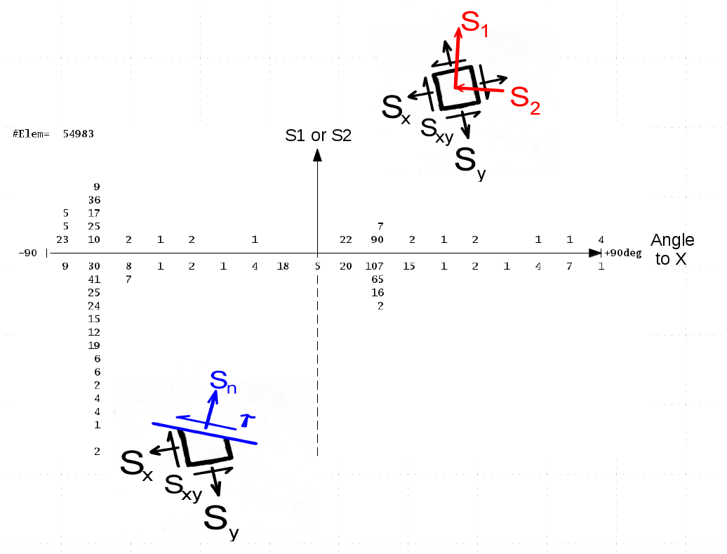
Fig. 5:
Values computed for S1 and S2 and their associated angles from the X axis are
plotted in a matrix of occurrences as shown in the middle of the figure for a short
load history. Angles are divided into 10 degree intervals. The angle interval
with the largest stress fluctuation (or some other criterion) is then selected to
be the direction with the most fatigue damage. A cut is then assumed in the
element at 90 degrees to this critical direction and the stress history ( Sn )
on that plane is computed with subsequent Rainflow cycle counting and a uniaxial
fatigue analysis.
Fatigue Analysis:
It is common practice to write the results of the fatigue analysis, and maximum
stress directions etc to a PATRAN or other type file for graphical display.
The fatigue analysis for a given element, however, is computed by the same
uniaxial fatigue life calculation program such as
saefcalc2.f.
Computationally this would be the most expedient, but other programs such as
a crack propagation program could also be applied.
References:
- [1] F.A.Conle and C.W.Mousseau, "Using vehicle dynamics simulations and
finite-element results to generate fatigue life contours for chassis
components," Int. J. Fatigue, V 13, N3, 1991, pp.195-205.
- [2] H.Agrawal, A.Conle, et al."Upfront Durability CAE Analysis for
Automotive Sheet Metal Structures, SAE Paper 961053, Feb. 1996.
- [3] C.-C. Chu, "Multiaxial fatigue life prediction method in the ground
vehicle industry," Int. J. Fatigue V 19, Supplement N1, 1996, pp.S325-S330.
- [4] C.C. Chu, F.A.Conle, A.Huebner, "An Integrated Uniaxial and Multiaxial
Fatigue Life Prediction Method," VDI Bericht Nr. 1283 1996, pp.337-348.
- [5] "SAE Fatigue Design Handbook," SAE AE-22, 1997 ISBN 1-56091-917-5
- [6] "Mulatiaxial Fatigue of an Induction Haredened Shaft," SAE AE-28,
Editors: T.Cordes and K.Lease, 1999, ISBN 0-7680-0528-0
- -
- Various commercial versions:
- FEMFAT Software:
link
- FE-SAFE Software:
link
- NCODE Software:
link