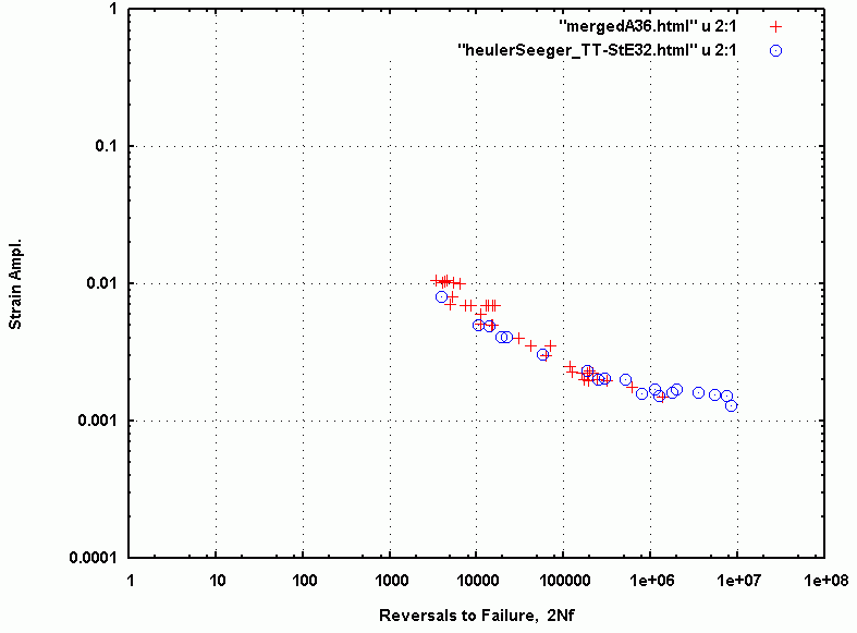
Fig. 1: Comparison of TT StE 32 and A36 Steel strain-life data.
For crack initiation calculations the program
saefcalc2.f
is applied. It uses the common
ground vehicle approach of a strain-stress-life curve from axial sample tests to
model the stress-strain and fatigue behavior, and a
Neuber plasticity correction
to translate Elastic Analysis Rainflow cycle counted loads into local
stresses and strains for crack initiation predictions.
The crack propagation program also accounts for material memory on a
half-cycle by half-cycle basis and for crack propagation calculations applies
the BS7910-2005 design guidelines.
The bottom flange steel is described as a BHW-25 (DIN 1.8802), while the web is
designated as a TT-StE32 (DIN 1.0851). It was not possible in the present work
to find the chemistry for these two steels nor an equivalent AISI or SAE designation.
Heuler and Seeger, however, do provide graphs of strain controlled fatigue test
results for specimens cut from the two steels and for the weld metal that joins
them. Data for the two steels and the weld metal are given in the files located
here.
Heuler and Seeger observed both crack initiation and propagation life of the
component, but no crack propagation information was found in the internet for
these steels. It was therefore necessary to find an approximate match to a
material for which crack propagation data was available. In figure 1 below
a comparison plot of the web TT StE32 beam web material is made for the strain-life
data points of
A36 structural steel. [Refs. 3-8] and another comparison is made for
Neuber equivalent
stress in figure 2. Figure 3 compares the cyclic stress-strain data points of
the two steels.
Fig. 1: Comparison of TT StE 32 and A36 Steel strain-life data.
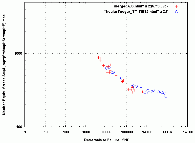
Fig. 2: Comparison of TT StE 32 and A36 Steel data for Neuber Equivalent stress.
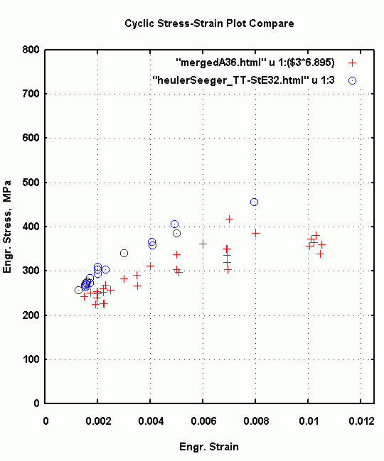
Fig. 3: Comparison of TT StE 32 and A36 Steel Cyclic Stress-Strain points.
In the comparison plots above one can observe that the TT StE32 point are slightly
above the A36 data points. Allowing for typical scatter observed in similar steels[2]
it was concluded that A36 steel is similar enough in its fatigue behavior that we
can use the A36 crack propagation data generated for the "Total Life" project of
the F.D.+E. Committee[3].
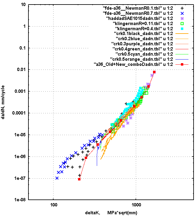
Fig.4: Crack propagation rate plot of measurements on A36 and other
steels with manually fitted curve shown in red. Refs.[4-8]
The square red points in figure 4 were fitted visually to the general
trend of the data. Table 1 shows the digitized points.
     #               Table 1   (file= a36_Old+New_comboDadn.tbl )

     # A36 101x101mm bar crack propagation data.
     # Digitized points manually from graph a36_Old+New_comboDadn2.png
     # which is a combination of low carbon steel  dadn plots
     # plus the A36 data from Newman and from the FDE  A36 101x101mm bar.
     #
     #Name= A36+LowCarbonFitted
     #deltaKunits= mpa_mm
     #dadnunits= mm
     #
     # deltaK    dadn
     # Mpa_mm     mm/cyc
     206.98 9.08542e-08
     248.243 8.7709e-07
     345.264 3.56202e-06
     486.714 1.3534e-05
     663.402 4.60083e-05
     960.    0.00020
     1175.75 0.000531564
     1419.67 0.00168951
     1667.   0.0077
#                              Tabel 2
#
#                    ( Loads normalized to +/- 1.0 )
#
#                      MaxLoad  MinLoad  No.Cycles
                      0.65294 -0.633492      1
                      0.805247  0.101319  3250
                      0.490046  0.208638  1250
                      0.649607  0.184034  1250
                      0.488703  0.257532  5000

                      0.757659 -0.249018     5
                      0.607893  0.197187  5000
                      0.490535  0.257063  5000

                      0.757659 -0.249018     5
                      0.607893  0.197187  5000
                      0.490535  0.257063  5000

                      0.757659 -0.249018     5
                      0.607893  0.197187  5000
                      0.490535  0.257063  5000

                      0.757659 -0.249018     5
                      0.607893  0.197187  5000
                      0.490535  0.257063  5000

                      0.757659 -0.249018     5
                      0.607893  0.197187  5000
                      0.490535  0.257063  5000

                      0.491354  -0.72443     2
                     -0.0607181 -0.724218    5
                      0.878091   0.180459    1

                      1.00097  -0.628375    10
                      0.808077 -0.43718    100
                      0.712938 -0.34584   1000
                      0.517959 -0.147447  3000
                      0.420928 -0.0603698 5000
                      0.333058  0.043123 10000
Each sub-block of cycles was then expanded using a Fortran program
(available here )
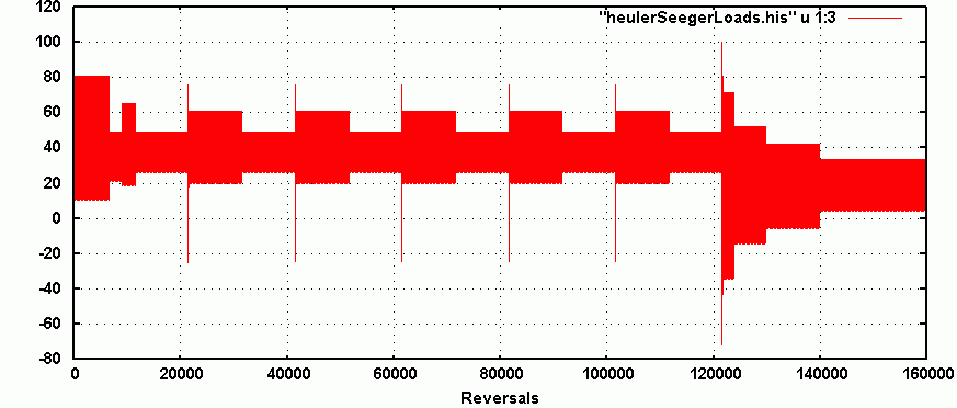
Fig.5: Load history scaled to +/- 100
When regenerating a block loading history from sets of sub-blocks it is important
to understand that the transition cycles that join adjacent sub-blocks are recognized
for both testing and simulation purposes. Thus one cannot simply add the simulated
damage of each block to make predictions. A better practice is to recreate the test
history and then Rainflow cycle count the results for crack initiation simulations and
to simply use the whole test history for crack propagation computations.
For testing and half-cycle by half-cycle simulations it is also important to get
the block to block transitions correct. In the complete history list linked
above there is no "zero" stress entered at the begining of the end of the complete
block history. The very first load application in both test and simulations would
of course start from zero load or stress, but subsequent end of block to start of
block transitions would not return to zero stress. In some high mean histories a
return to zero could be a significantly damaging cycle, and the history user needs to
be aware of the potential problem. Three magnifications of portions of the history
are presented in the following three figures.
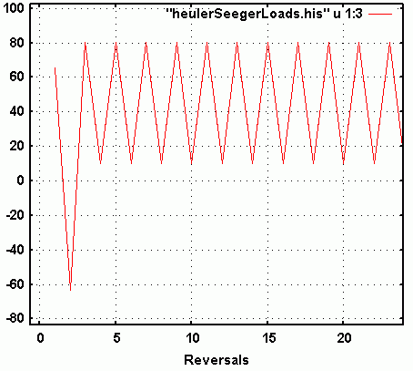
Fig.6: Initial load cycles of the history.
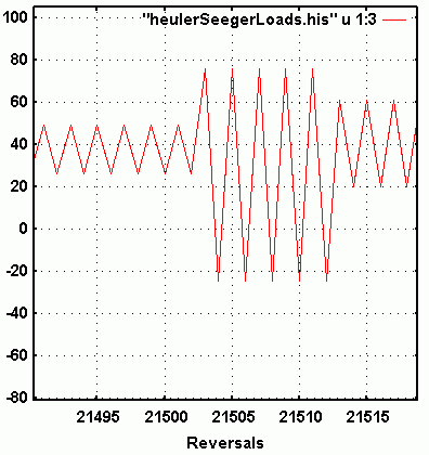
Fig.7: A transition section in the history.

Fig.8: A transition section in the history.
The load history shown in figure 5 has a tensile mean as shown. The loads were applied
to the component such that the bending stresses at the 55deg notch (Kt=2.3) had a
compressive mean, and the 125deg notch (Kt=1.5) had a tensile mean.
From crack surface marks it was possible to count back to the cycles at which the cracks
were approximately 1 to 2 mm in size. This crack size initiated at history repetition no. 18.
The authors also subjected unnotched axial samples to the notch strain histories, a process
termed "companion specimen" testing, which yielded lives similar to component initiation life.
Initiation Simulation:
Links to the open source crack initiation software saefcalc2.f are found
here.
The program uses a "fitted" digitally described strain-stress-life curve to
compute fatigue damage of local stress-strain hysteresis loops at the fatigue hot spot.
For welded components, where weld metal distorts the base metal properties, a generic
fitted strain-stress-life curve for
A36 steel is used to compute damage.
The non-periodic overstrain fitted strain-stress-life curve is available
here.
For variable amplitude tests it is common practice to expect fatigue
damage from small cycles that under constant amplitude conditions would
be under the fatigue limit. Periodic overload or overstrain (POL) data
for A36 are not available. Based on experience with other data sets the
red line with points, shown in figure 10 are the expected POL strain life
curve. The file of fitted data points for A36 POL is located
here.
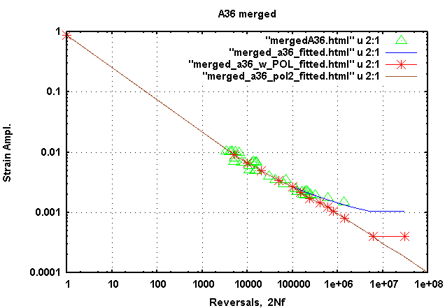
Fig. 10: Estimated periodic overload effect on the strain life curve for A36 Steel.
A similar POL effect curve was created for the weld metal tested by Heuler and Seeger.
Figure 11 shows the estimated POL curve and the original constant amplitude (CA) strain
life curve. The fitted points used for damage computations are located
here.
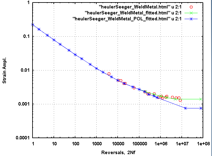
Fig. 11: Estimated periodic overload effect on the strain life curve for weld metal.
Crack initiation life prediction were made with the regular CA curves and
with the POL curves for the history described above. A Kt=-2.3 was applied
to the Rainflow counted data sets. The "-" sign in front of the 2.3 effectively
"flips" the history such that tensile maxima become compressive and vice versa.
The Linux bash shell script to automatically run all the crack initiation
predictions and make the reports is located
here. In this study it was
activated with the command:
./runKt -2.3
(after removal of the ".txt" suffix.)
The initiation prediction results when one uses the CA fitted curves and the
POL fitted curves differ by factors of approximately 1.5 to 2.0 , which is
a substantial difference. Normally POL curves are used to predict life
of highy variable histories such as the
Grapple Skidder Torsion
history.
In such cases one automatically defers to the POL results. In the case of
the present "sub-block" history there are however substantial numbers of CA cycles.
It is not immediately clear if POL should govern.
 Click to enlarge
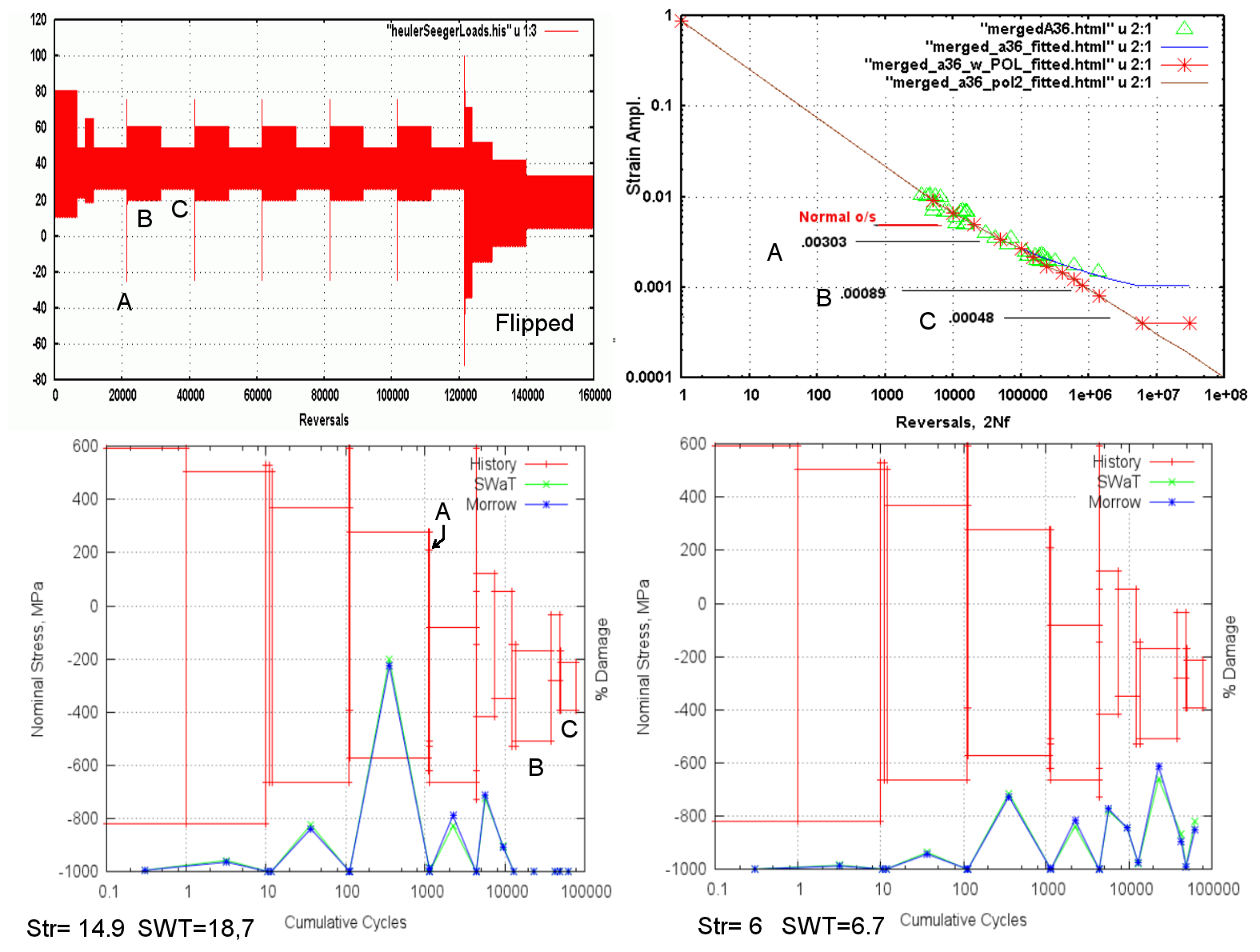
Fig. 12: Calculated damage for A36 CA fitted curves and A36 POL fitted curves.
Figure 12 shows the Heuler-Seeger history in the upper left region, and the CA and POL
fitted curves used to calculate damage. Sub-blocks labelled B and C would under CA
conditions not cause any fatigue damage. The Rainflow historgram and percent Damage
plots for predictions using the A36 CA fitted curve is shown in the lower left
region, while the POL results are depicted in the lower right figure. The percent
damage in blue and green along the lower boundary of the two figures show the
effect of presense(CA) or absense(POL) of the fatigue limit at the right side of
the percent damage plots.
It is necessary to determine whether one should use CA or POL fitted curves
in histories, as in the present study, that consist of numerous CA sub-blocks.
In order to activate the POL effect two features must be present in the local
hot spot stress-strain history of the component.
    1. The larger cycles must be big enough to cause the POL effect;
       typically of a size that would, under CA conditions, result in
       a life around Nf=10000.

    2. The larger cycles must occur often enough that the effect
       does not dissipate during application of the smaller cycles.
DuQuesnay et al [9] have calculated how many of the smaller cycles are needed
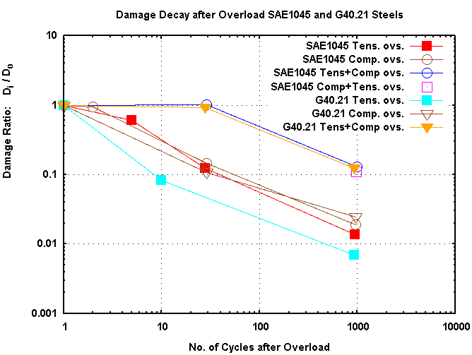
Fig. 13: Decay of damage for small cycles that follow an overload.
( TC=Tension-Compression overload; T=tensile overload; C=compression overload )
Figure 14 shows the sum, at any subsequent small cycle, of the damage fractions of
the small cycles up to that point.
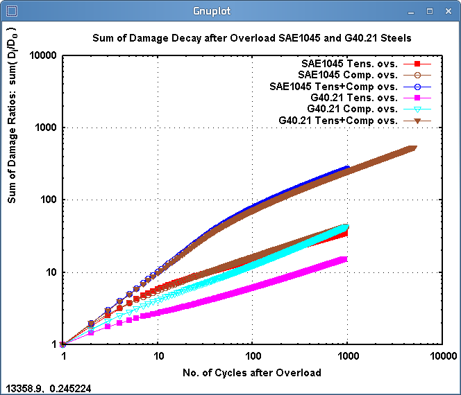
Fig. 14: Sum of damage fractions for small cycles that follow an overload.
( TC=Tension-Compression overload; T=tensile overload; C=compression overload )
When one sums these damage fractions of the smaller cycles, as for sub-block B
in the above, one can compute the number of fully POL equivalent damaging cycles.
For the 5000 cycles of sub-block B, that have damage fractions equal to 1 or less,
the same amount of damage would be done by 550 fully POL damaging cycles.
One can thus change the cycle numbers in the Rainflow count file to reflect these
reduced cycle numbers and re-calculate the predicted crack initiation life.
This process has been applied to the predictions documented in the following
two reports:
Summary of Crack Initiation Predictions:
                     Initiation Block Life Results

 Predictions:
                    StrainLife      SWT        Morrow

       A36             14.9         18.7         19.7

       A36+POL          6.0          6.7          6.9

     A36+POL-Decay     10.0         12.5         12.7


    Weld Metal         34.7         43.8         34.7

   WeldMetal+POL       20.0         24.2         26.6

 WeldMetal+POL-Decay   24.1          29.9        32.3


Test Results:
                         Crack
                       Initiation         Fracture
                       (1 to 2mm)
  Component Test            18               21


  Axial Companion
   Specimens             14 to 18         17 to 20
Given all the considerations mentioned in the above sections its is the
Blocks to initiation = 24.1
Other run-time files are:
Results: